---
title: "1. Figures and statistical tests using eDNA data"
subtitle: "Building on group eDNA projects"
page-layout: article
author:
- Amy Van Cise
- Sarah Tanja
date: "2026-02-12"
draft: false
date-modified: today
order: 1
format:
html:
toc: true
toc-depth: 2
number-sections: false
code-fold: true
editor:
markdown:
wrap: 72
---
```{r setup, include=FALSE}
knitr::opts_chunk$set(
echo = TRUE,
message = FALSE,
warning = FALSE
)
```
# Background
This week you will continue to work in your groups to build upon your
final lab project using the eDNA dataset!
The focus in this lab will be polishing up your figures and performing
statistical tests to answer your specific research question. You will
continue to write up your findings in a lab report format *with
citations*!
> A note about statistical tests: So far this quarter, we've looked at
> research questions that can be answered with an ANOVA or a linear
> regression. For the major lab project, the required statistic is an
> ANOVA or linear regression. If you learned a statistical test or model
> in another class that you want to apply here, I encourage you to try
> it out!
# Week 7 Lab Report should include:
1. Background information on chosen predator (e.g. diet, distribution,
habitat use, competitors, predators) ***with MORE context relating
to your specific hypotheses and findings, backed up with references
using inline citations***
2. Citations **use the default [Chicago Manual of
Style](https://www.chicagomanualofstyle.org/home.html) author-date
format**
3. Finalized Broad Research Question
4. Finalized Specific Research Question (if needed)
5. Finalized Falsifiable Null and Alternate Hypotheses (be specific)
6. Defined X and Y variables
7. **Figure(s) showing X and Y variables for each hypotheses tested**.
8. **Statistical test results, and a statement about whether you reject
or fail to reject the null hypothesis.**
9. **Draft paragraph reflecting on your results and how your group
interprets them. What is the story behind the data?**[^1]
[^1]: New elements expected to be added for your week 7 iterative report
are in **bold**
```{r, include=FALSE}
library(tidyverse)
library(colorspace)
```
```{r, include=FALSE}
eDNA <- read_csv("../../week5/data/eDNA_MM_fish_detections_clean.csv")
```
```{r}
humpy <- eDNA %>%
  filter(common_name == "humpback whale") %>%
  pivot_longer(16:length(.), names_to = "prey_species", values_to = "prey_prop") %>%
  group_by(Detected, prey_species) %>%
  filter(mean(prey_prop) > 0.01) %>% # !!!!
  ungroup()
```
```{r}
humpy_Sleucopsarus <- humpy %>%
  filter(prey_species == "Stenobrachius leucopsarus")
```
# Polish your figure(s)
#### Explore the types of plots you could make in the [R graph gallery](https://r-graph-gallery.com/)
::: callout-important
Pick at least one plot or figure that illustrates your X and Y variables
from *each* set of tested hypotheses
:::
#### Choose a color palette
[PNWColors](https://github.com/jakelawlor/PNWColors)
- `rev()` reverses the order the colors are assigned
```{r}
library(PNWColors)
mycolors <- rev(pnw_palette("Bay", 2, type = "discrete"))
```
- `scale_color_manual()` controls the outline of your geom
- `scale_fill_manual()` controls the fill of your geom
#### Plot title and axis labels
- `labs()` cotrols the following
- `title = "X vs. Y"` plot title
- `x = "X variable label"` x axis label
- `y = "Y variable label"` y axis label
#### Explore the different [built in themes](https://ggplot2-book.org/themes.html#sec-themes)
You can try:
- `theme_minimal()`
- `theme_grey()`
- `theme_bw()`
- `theme_classic()`
You can customize other parts of your plot in the `theme()` call if you
choose... download this pdf theme cheatsheet if you want to learn more
about it!
<object data="../refs/ggplot theme system cheatsheet.pdf" type="application/pdf" width="100%" height="500px">
<p>Unable to display PDF file.
<a href="../refs/ggplot theme system cheatsheet.pdf">Download</a>
instead.</p>
</object>
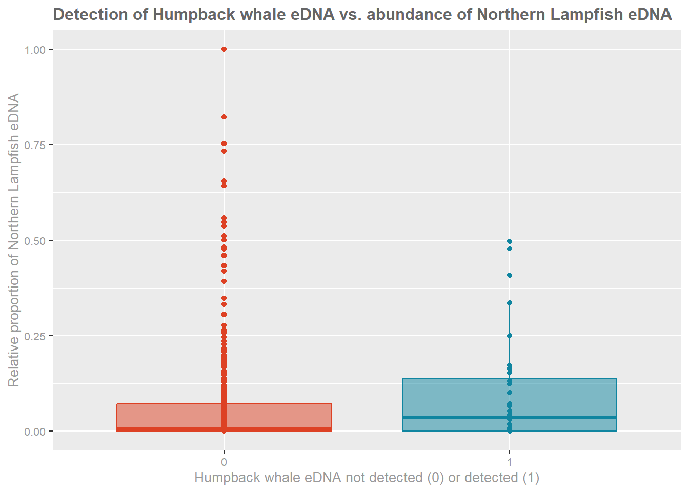
#### Example figure:
```{r}
ggplot(humpy_Sleucopsarus,
       aes(x = prey_prop,
           y = as.factor(Detected),
           fill = as.factor(Detected),
           color = as.factor(Detected))) +
  geom_point() +
  geom_boxplot(alpha = 0.5) +
  coord_flip() +
  scale_color_manual(
    values = mycolors,
    name = "Humpback Whale eDNA",
    labels = c("Not detected", "Detected")
  ) +
  scale_fill_manual(
    values = mycolors,
    name = "Humpback Whale eDNA",
    labels = c("Not detected", "Detected")
  ) +
  theme_grey() +
  labs(
    title = "Detection of Humpback whale eDNA vs. abundance of Northern Lampfish eDNA",
    x = "Relative proportion of Northern Lampfish eDNA",
    y = "Humpback whale eDNA not detected (0) or detected (1)"
  ) +
  theme(
    legend.position = "none",                    # 🔹 hide key
    axis.text = element_text(size = 8, color = "grey60"),
    axis.title = element_text(size = 10, color = "grey60"),
    plot.title = element_text(size = 12, color = "grey40", face = "bold")
  )
```
# Choose your statistical test
##### 1. Identify your predictor variable(s) based on the wording of your specific hypothesis

##### 2. Are your predictor variables categorical or continuous
::: callout-tip
If your predictor variable (x) is categorical –\> your model is an ANOVA
If your predictor variable (x) is continuous –\> your model is a Linear
regression
:::
# Run your statistical test
## ANOVA
A one-way ANOVA in R tests whether the **means of a continuous response
(y) variable differ across your categorical predictor (x) variable of
two or more groups**. Conceptually, it asks: *Is the variation between
group means larger than we would expect from random variation within
groups?* In R, you typically run it with
`aov(y ~ group, data = your_dataframe)`
::: callout-tip
Read up on the usage of the built in ANOVA function `aov()` from the
`stats` package by running `?aov` in the console or a code chunk
:::
```{r, eval=FALSE}
?aov
```
```{r}
anova_res <- aov(prey_prop ~ Detected, data = humpy_Sleucopsarus)

summary(anova_res)
```
```{r}
humpy_Sleucopsarus %>%
  group_by(Detected) %>%
  summarise(mean(prey_prop))
```
## Linear regression
A linear model in R using `lm()` estimates the relationship between a
**continuous response (y) variable** and one or more **continuous
predictor (x) variables**. At its core, it fits a line that minimizes
squared residuals.
::: callout-tip
Read up on the usage of the built in linear model function `lm()` from
the `stats` package by running `?lm` in the console or a code chunk
:::
```{r, eval=FALSE}
?lm
```
```{r}
lm_res <- lm(Detected ~ prey_prop, data=humpy_Sleucopsarus)
summary(lm_res)
```
# Report, Reject or Accept... & Interpret!
##### ANOVA
In an ANOVA, the key outputs to report include the **group means**, the
**F statistic** and its associated **p-value**.
The F statistic is a ratio: $$
F = \frac{\text{variance between groups}}{\text{variance within
groups}}
$$ Your F statistic will be higher when the variance between groups is
large relative to the variance within groups, which suggests that the
group means are different.
The p-value tells you the probability of observing the F statistic
calculated from your data, assuming the null hypothesis is true (i.e.,
all group means are equal).
If the p-value is below your significance threshold (a default value is
typically ( $\alpha = 0.05$ )), you reject the null hypothesis that all
group means are equal.
::: callout-important
Importantly, ANOVA tells you **that at least one group differs**, not
*which* groups differ.
:::
An example for reporting ANOVA results:
> The mean proportional relative abundance of *Stenobrachius
> leucopsarus* eDNA in samples where humpack whale eDNA was not detected
> is 0.06, and 0.08 for samples where humpback whale eDNA was detected.
> A one-way ANOVA showed no significant difference in mean
> *Stenobrachius leucopsarus* eDNA proportional relative abundance
> between samples where humpback whale eDNA was detected and those where
> it was not detected \[F(1,514)=1.113, p=0.292\]. We therefore fail to
> reject the null hypothesis and find no statistical evidence that
> humpback eDNA detection status is associated with differences in
> lampfish eDNA abundance.
If the ANOVA is significant, you can follow it up with a **post hoc
test** like the Tukey Honestly Significant Difference test using the
`TukeyHSD(your_anova_result)` function to identify which specific pairs
of groups differ.
::: callout-tip
Interpret results in plain language: report the F statistic, degrees of
freedom, p-value, and group means — and always connect the statistical
result back to the biological or practical question you’re asking. You
should talk with your group about how you interpret your results in the
specific ecological context of what is known about your chosen predator,
prey, relating directly to your hypotheses!
:::
##### Linear model
After running `lm_res <- lm(y ~ x, data = your_data)` and
`summary(lm_res)`, make sure to report the **coefficients**: the
estimate tells you the direction and magnitude of the effect, the
**standard error** reflects uncertainty, the **t-value** is the
signal-to-noise ratio, and the **p-value** tests whether that
coefficient differs significantly from zero. The overall model
**F-statistic** tests whether the model explains more variation than a
null (intercept-only) model, and the **R^2^** reports the variance
explained by the model.
An example for reporting linear regression results:
> A linear regression was conducted to assess whether lampfish
> (*Stenobrachius leucopsarus*) eDNA proportional abundance predicted
> humpback whale eDNA detection. The model estimates a weak positive
> association, where higher lampfish eDNA proportional abundance
> corresponds to slightly higher predicted humpback detection
> probability; however, the magnitude of this effect is small and not a
> significant predictor of humpback detection status (β=0.0895,
> SE=0.0849, t(514)=1.06, p=0.292). The overall model was not
> significant \[F(1,514)=1.113, p=0.292\] and explained a negligible
> proportion of variance in detection status \[R^2^=0.002\]. Therefore,
> we fail to reject the null hypothesis that lampfish proportional
> abundance is associated with humpback whale eDNA detection.
::: callout-tip
When you interpret results, translate coefficients into meaningful
biological or practical terms — don’t just report significance; explain
what the estimated effect size actually means (ex. small positive
effect, large negative effect... describe the magnitude and direction of
the predictor variable effect on your response variable).
:::