This summary serves as a broad overview and notes of the acute (48hour) single stressor polyvinyl chloride (PVC) and polypropylene (PP) leachate exposure to Anthopleura elegantissima.
The following is a timeline overview of the experiment.
Note
Sample processing for Mitotic index, chlorophyll content, and DNA & RNA sequencing still have to be done!
This timeline was made using the vistime1 package
1 Checkout the vistime package vignette here
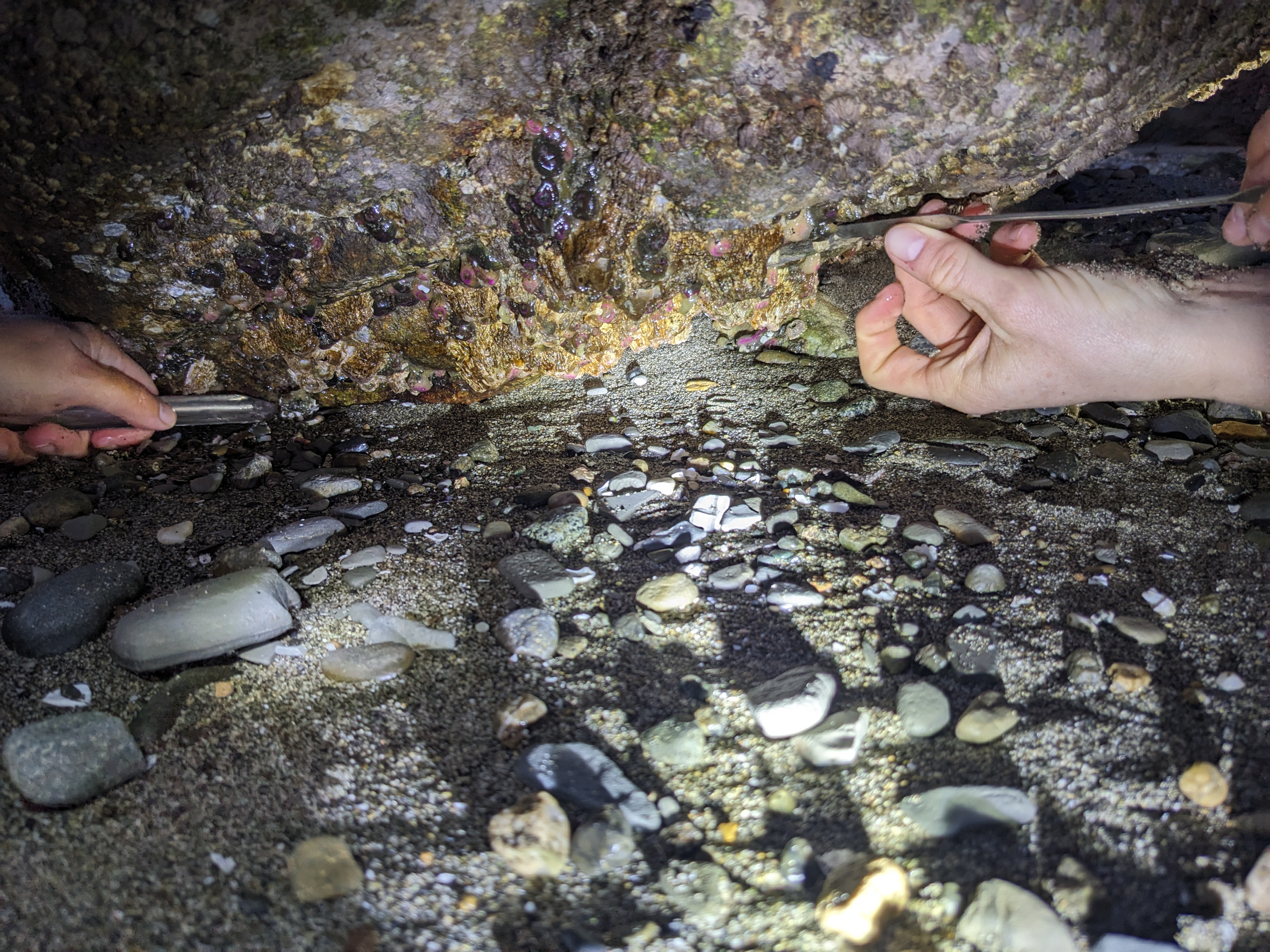
1 Specimen collection & acclimation
We collected anemones under Washington Dept. of Fish & Wildlife scientific collection permit Tanja-010 at Owens Beach Park in Tacoma on Monday March 18th and at Constellation Park in West Seattle on Saturday March 30th. After collection, each anemone was placed on a acid-washed 60mm glass petri dish to adhere and heal their pedal disc during an acclimation phase. All anemones were acclimated for at least 24 days in a recirculating seawater table at 10C prior to the start of the treatment exposure.
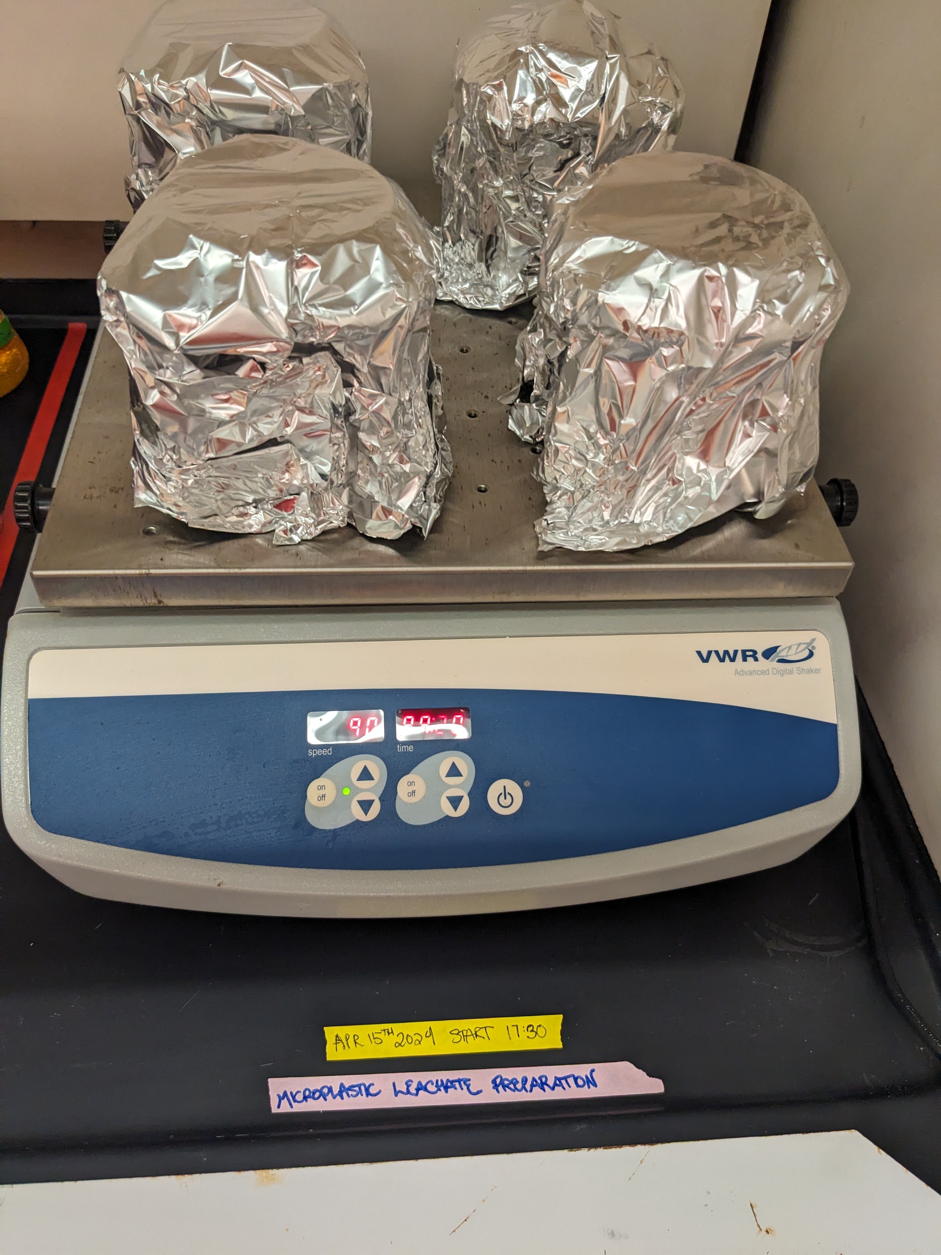
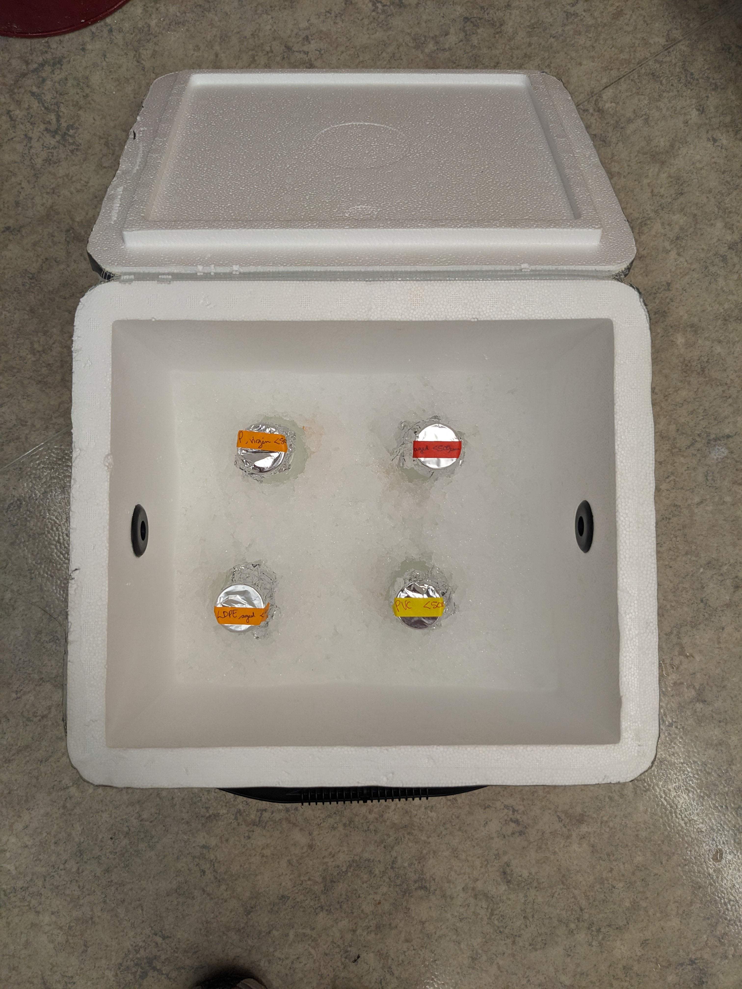
2 Leachate preparation
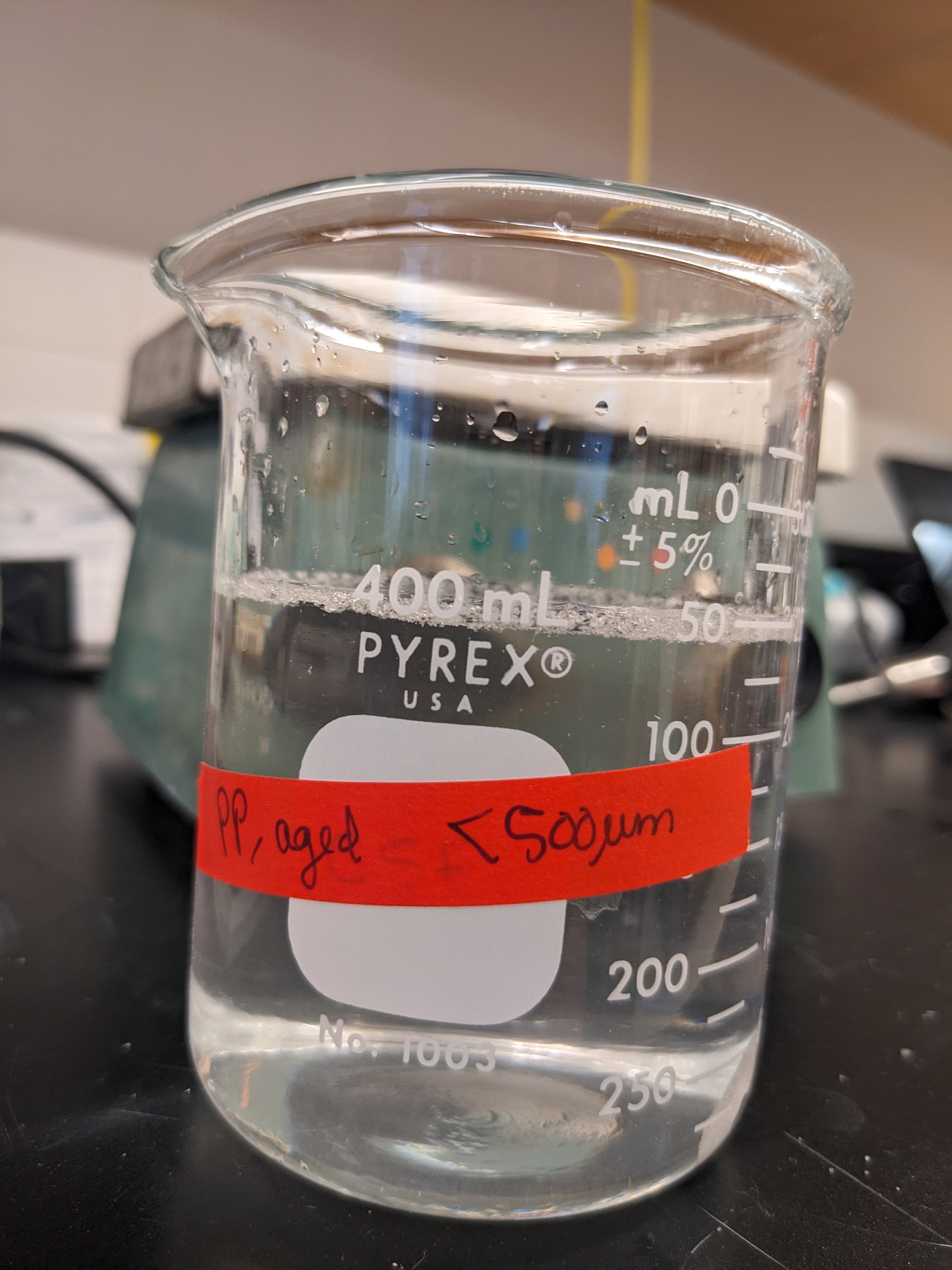
We prepared leachate for PVC (<500um) and for PP (aged) according to the leachate preparation protocol.
In short, we created 1L artificial seawater using salt and deionized water, and adjusted the pH down from ~8.5 to 8.2 by slowly, iteratively, adding a very small amount of 0.1M hydrochloric acid (HCl) via a burette.
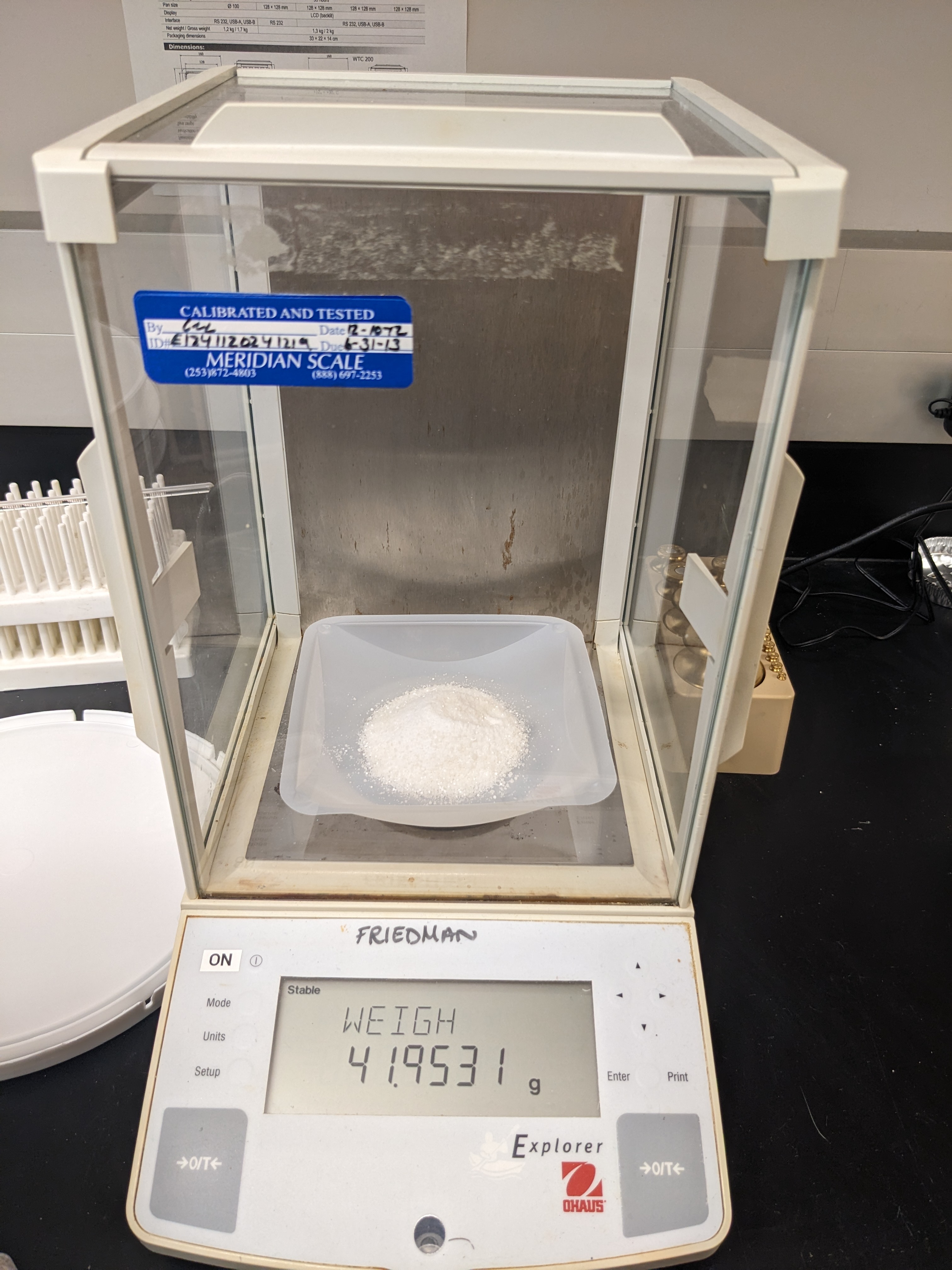
We then carefully measured out 250mg of each microplastic type, and added it to a dry flask.
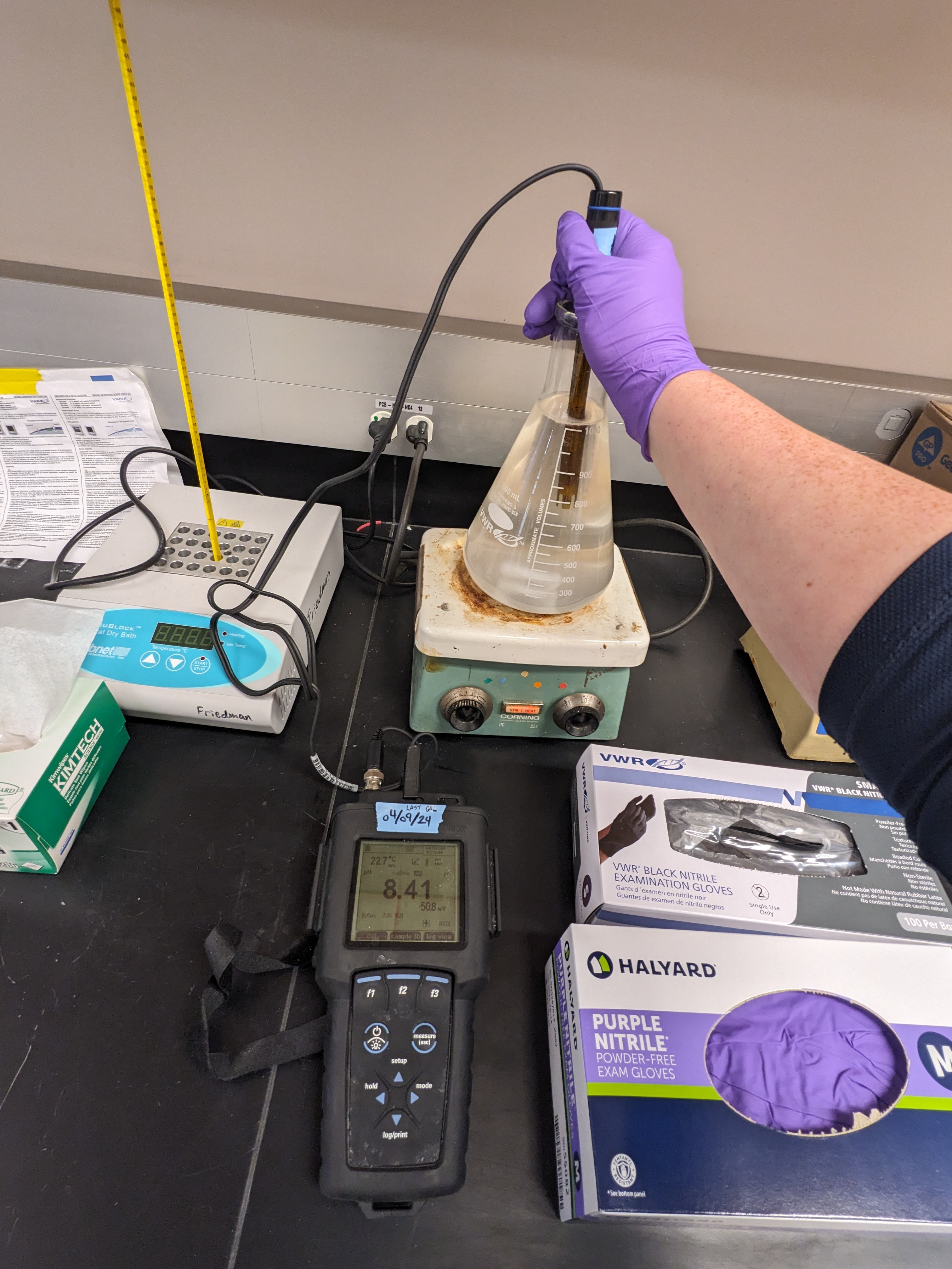
After, we transferred 250mL of the pH-adjusted artifical seawater to each flask, set them in a shaker plate rotating at 90 rotations per minute, and left them to ‘shake and soak’ for 7 days.
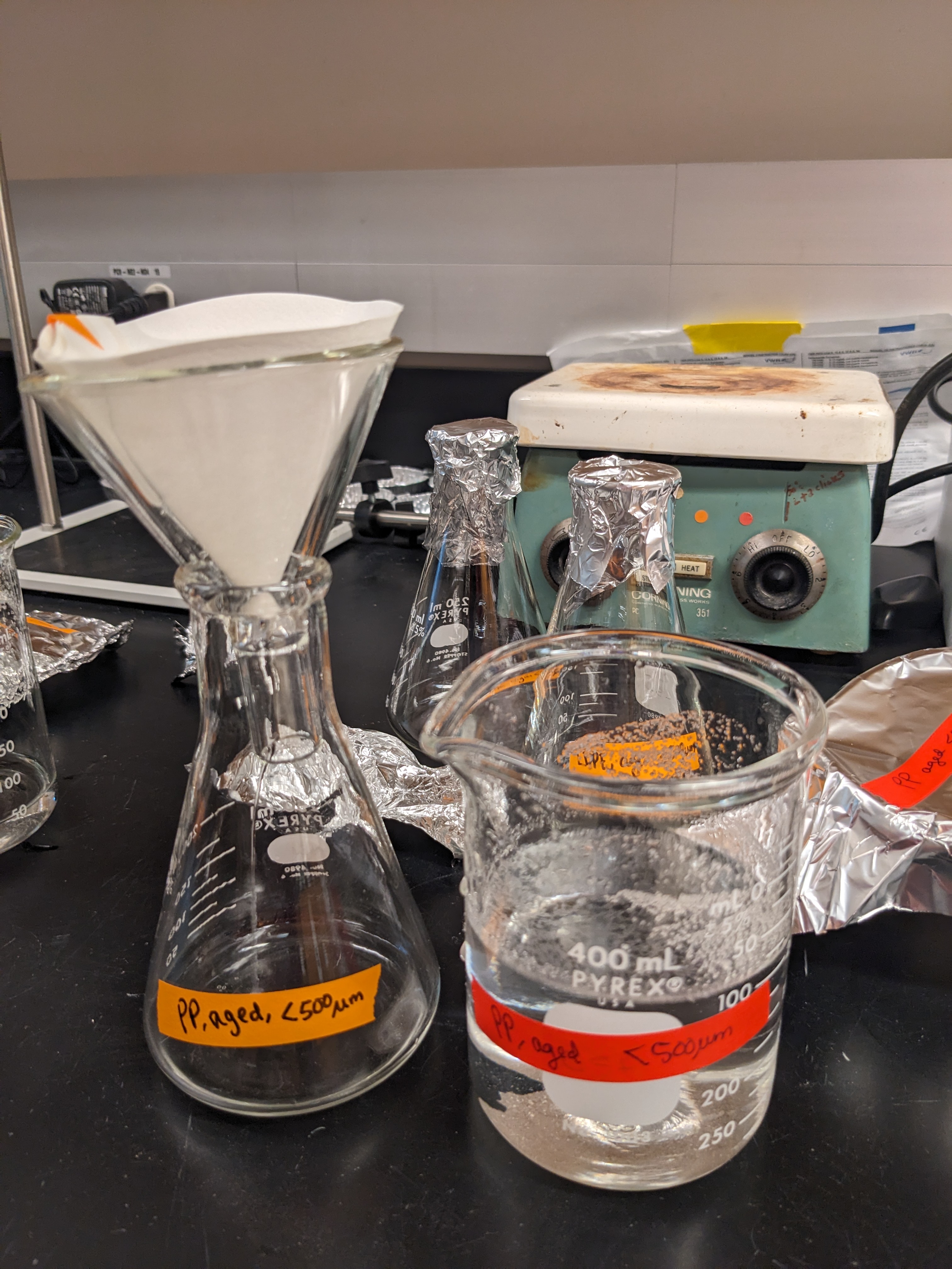
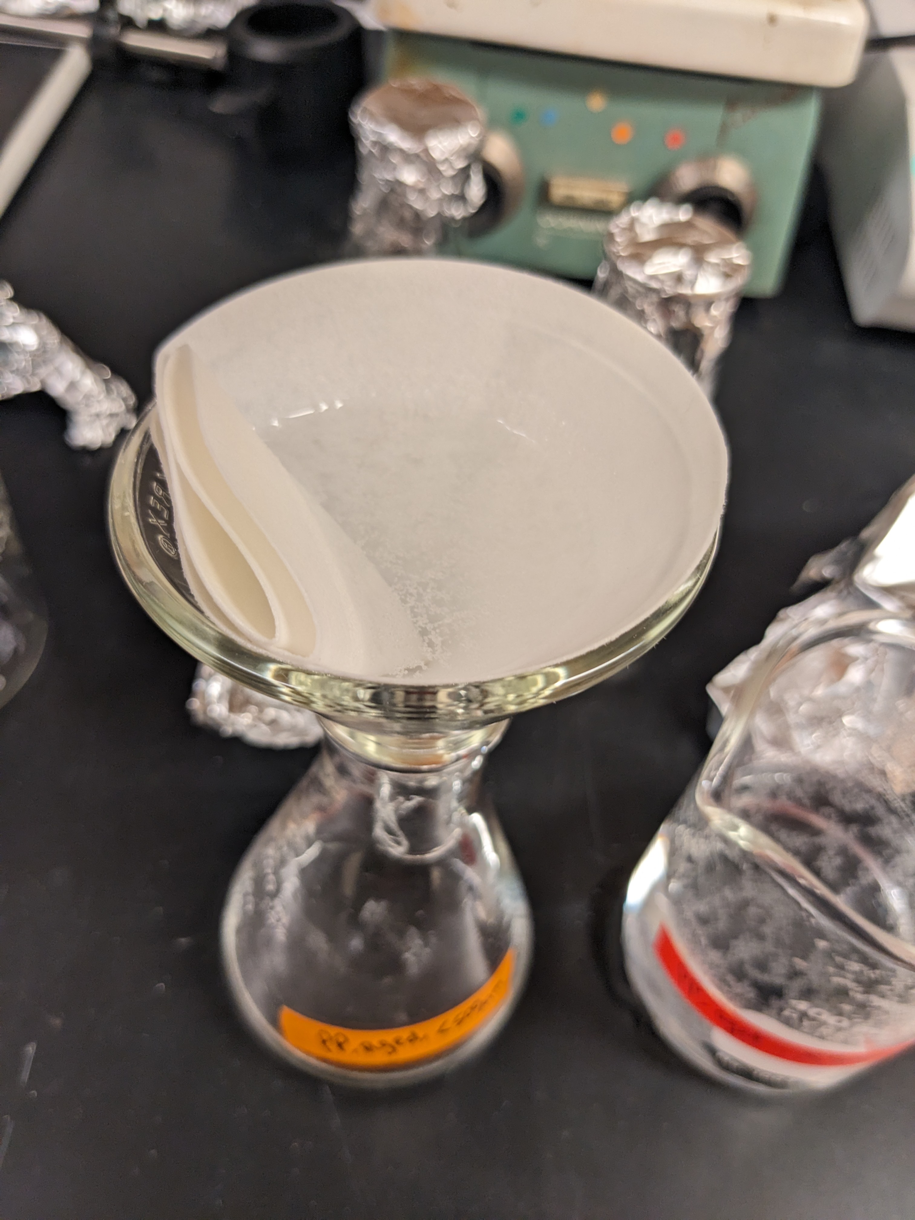
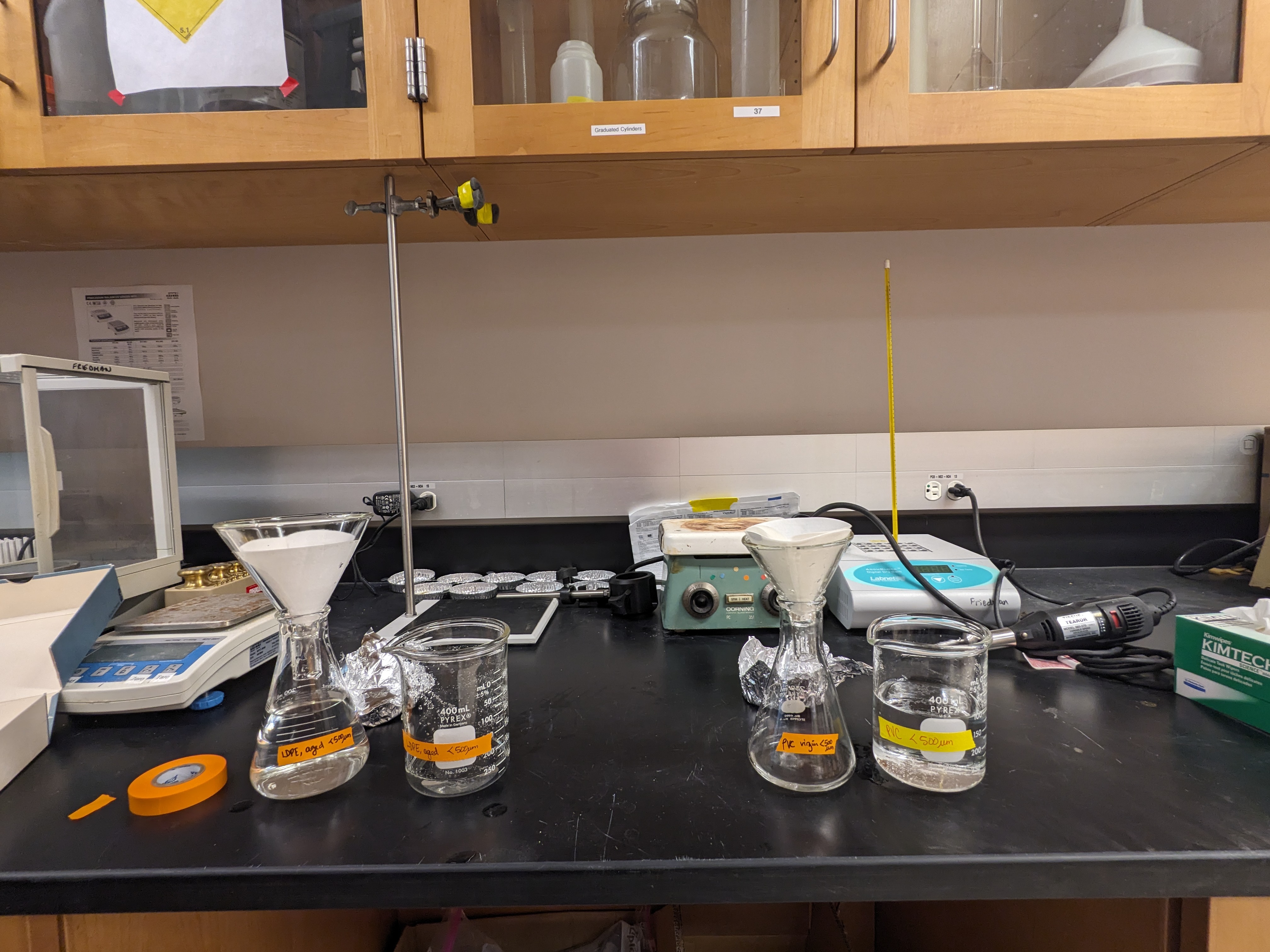
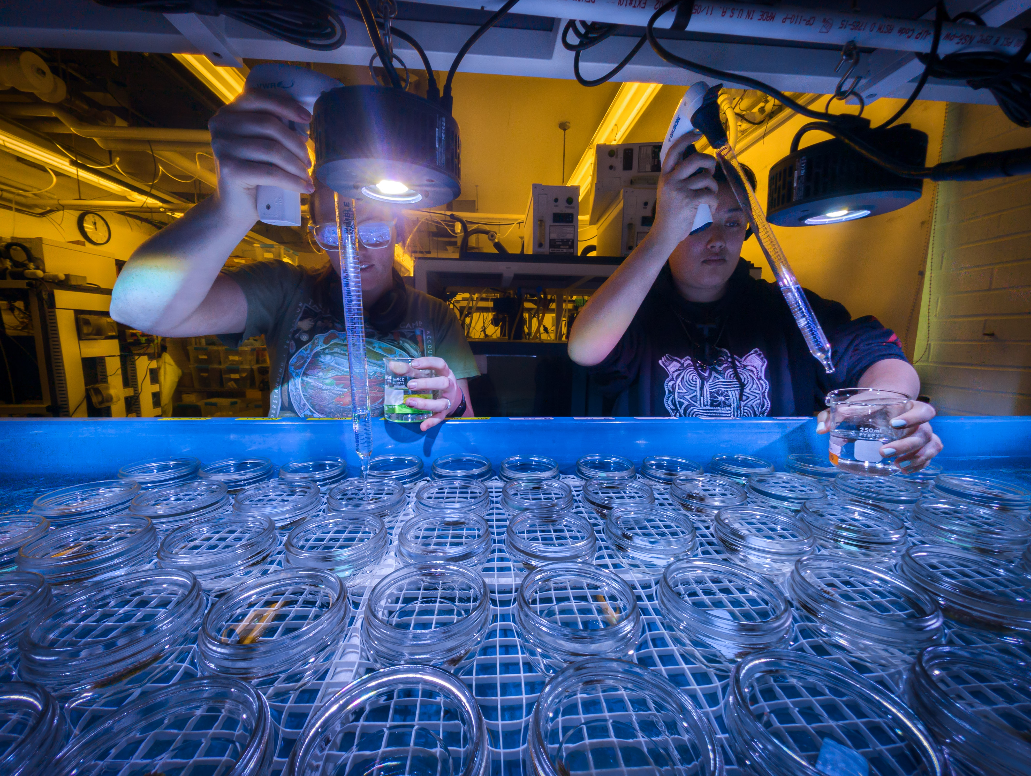
3 Leachate dilution
We performed a serial dilution on each prepared leachate to create leachate treatments that represent a mass of microplastic type to volume of water:
- 100 mg/L
- 10 mg/L
- 1 mg/L
- 0.1 mg/L
- 0.01 mg/L
For this we took 20mL of the 1000 mg/L leachate, and added it to 180mL of filtered seawater to make the 100mg/L concentration.
We then serially diluted the remaining concentrations in a similar fashion.
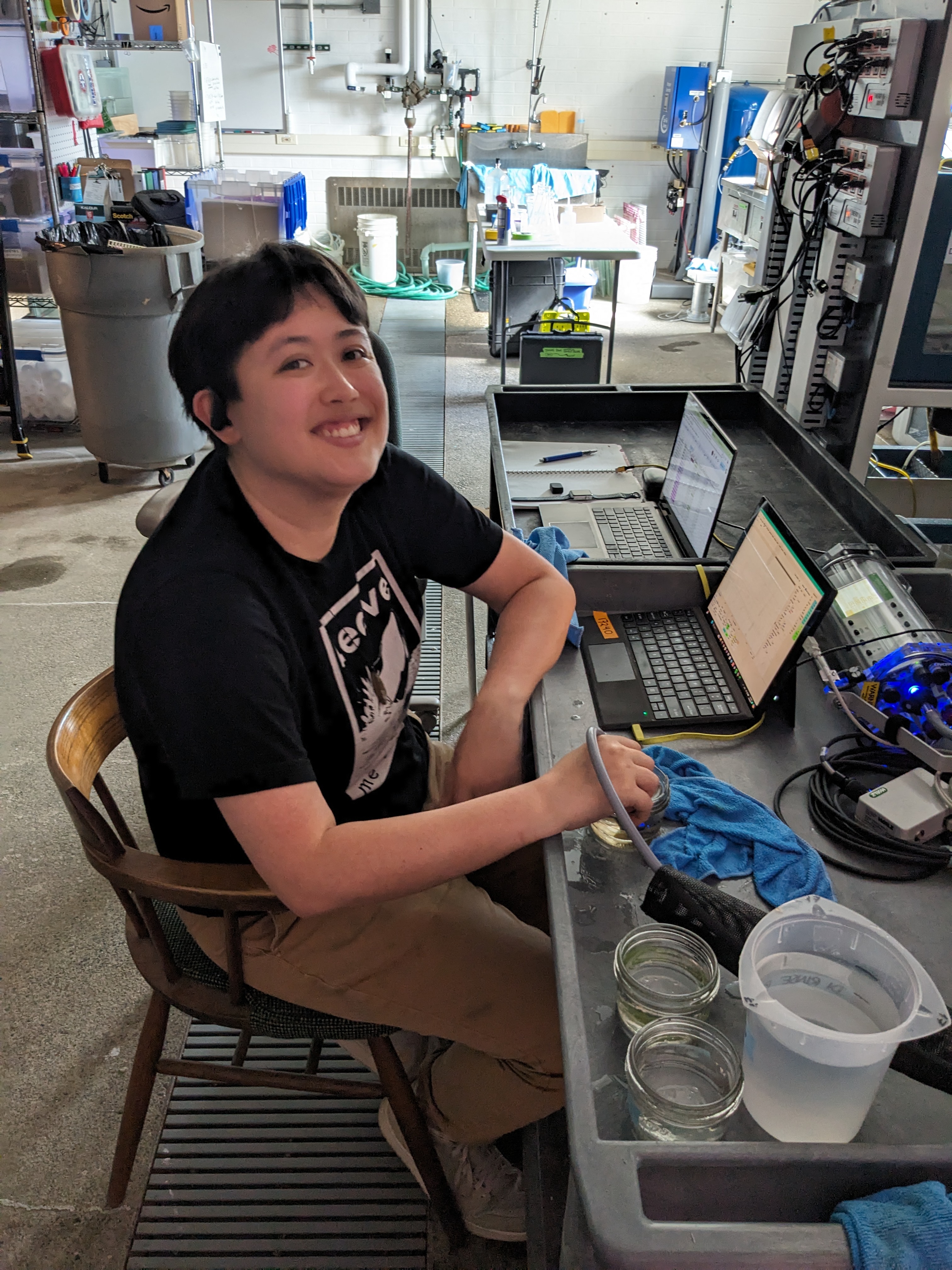
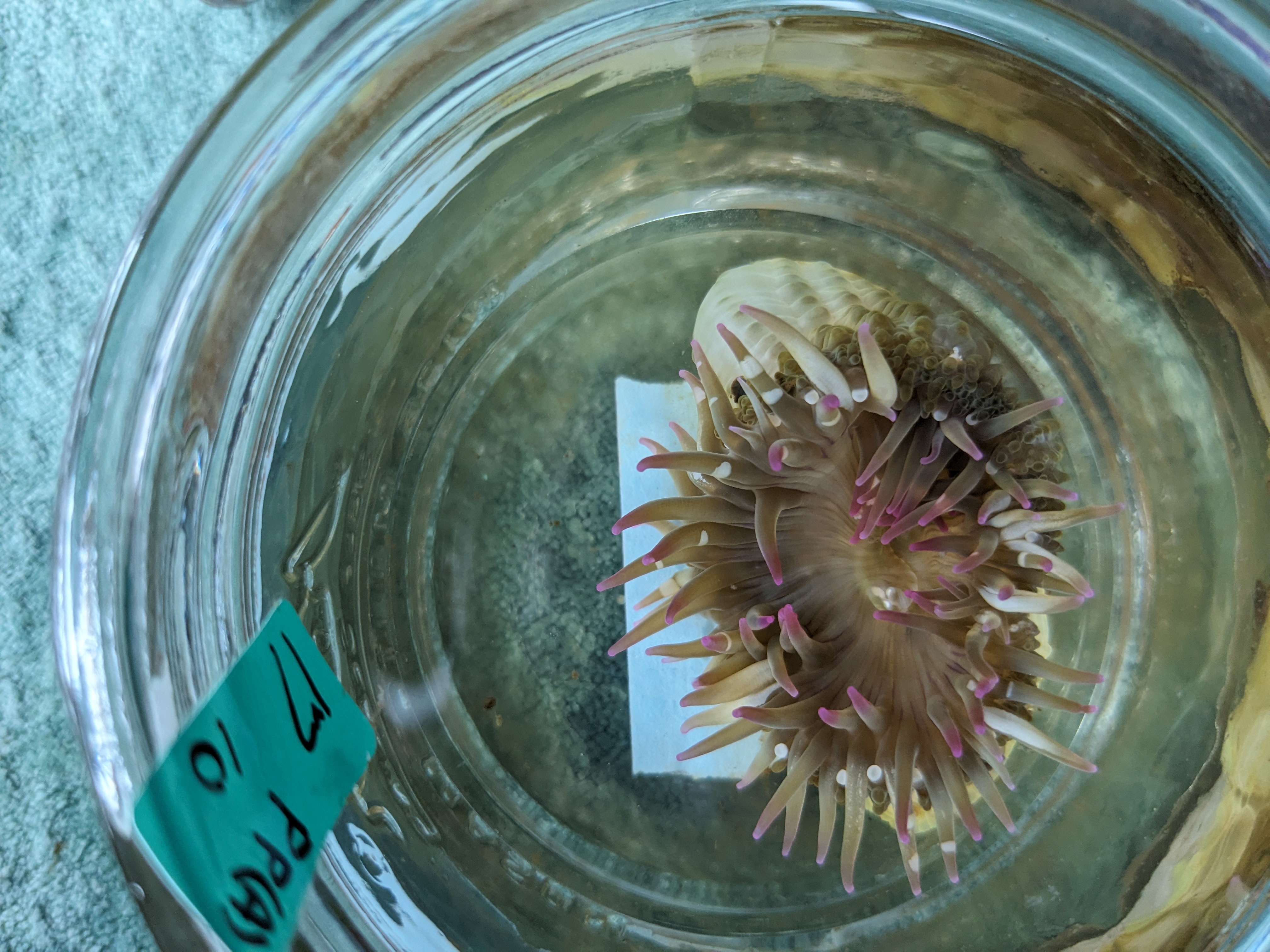
4 Exposure
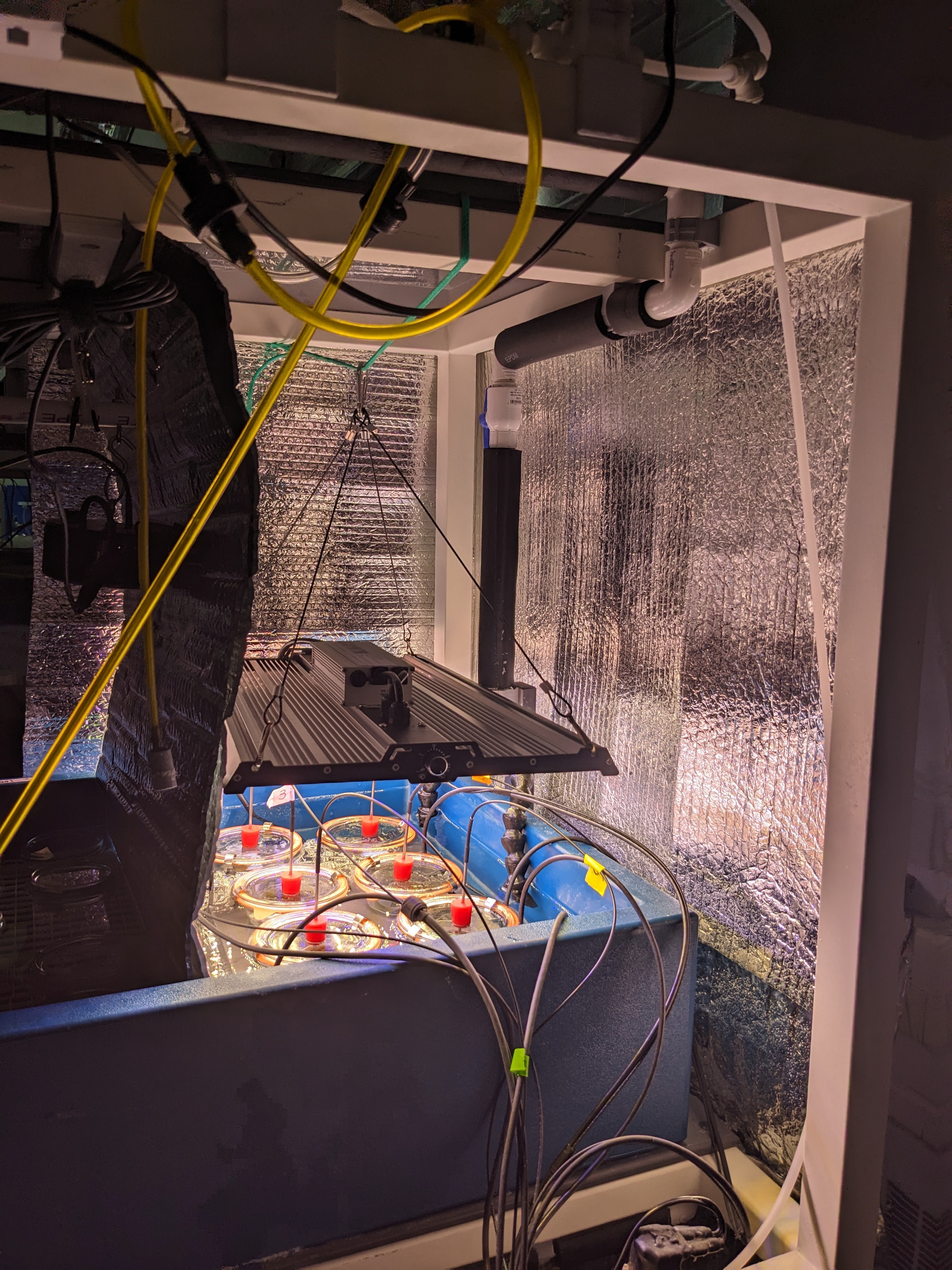
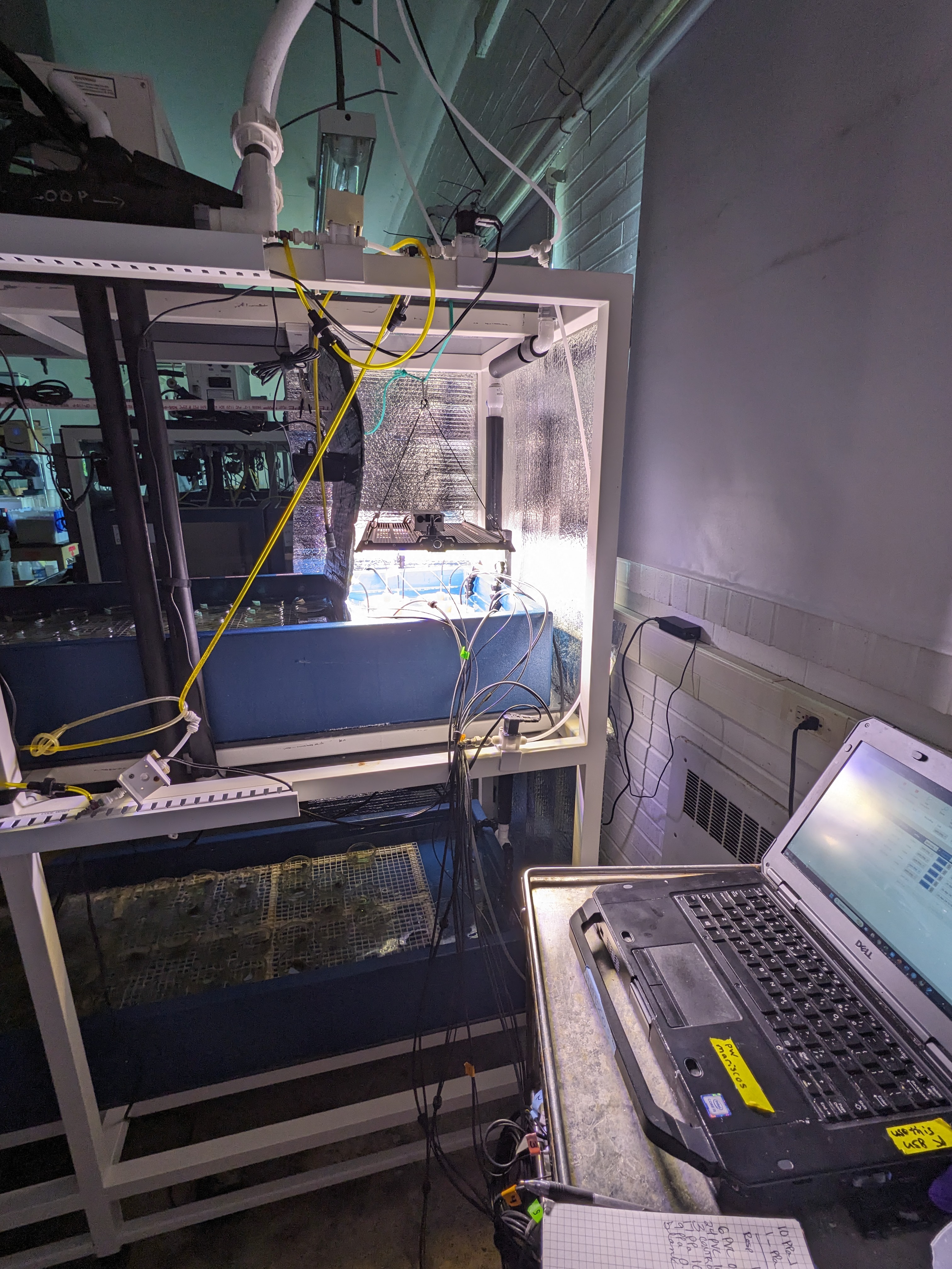
We exposed individual anemones to the leachate treatments for 48 hours in closed-systems. For this, we used 0.5 pint mason jars set in a recirculating seawater bath temperature-controlled by a heat exchanger and the Neptune Apex aquarium controller system.
The water bath was kept at 10C throughout the exposure.
5 Response measurements
After 48 hours we measured:
- Rapid Light Curves using a Walz Diving II PAM

30 minutes of respirometry in the dark-adapted state (oxygen consumption, cellular respiration)
30 minutes of respirometry in the light-saturated state (oxygen production, photosynthesis)
wet weight
And then placed anemones in labelled 5mL centrifuge tubes and flash froze them in liquid-nitrogen
6 Initial results
# Install packages
if ("tidyverse" %in% rownames(installed.packages()) == 'FALSE') install.packages('tidyverse')
if ("dplyr" %in% rownames(installed.packages()) == 'FALSE') install.packages('dplyr')
if ("car" %in% rownames(installed.packages()) == 'FALSE') install.packages('car')

# Load packages
library(dplyr)
library(tidyverse)
library(car)
Warning: package 'car' was built under R version 4.2.3Loading required package: carDataWarning: package 'carData' was built under R version 4.2.3
Attaching package: 'car'The following object is masked from 'package:dplyr':
recodeThe following object is masked from 'package:purrr':
somerates <- read_csv('rates.csv')Rows: 55 Columns: 17
── Column specification ────────────────────────────────────────────────────────
Delimiter: ","
chr (2): id, treatment
dbl (15): run, channel, auto_resp_rate, auto_resp_r2, resp_bg_adj.rate, resp...
ℹ Use `spec()` to retrieve the full column specification for this data.
ℹ Specify the column types or set `show_col_types = FALSE` to quiet this message.6.1 Respiration
6.1.1 First glimpse of data
ggplot(rates) +
  aes(x = treatment, y = massnorm_resp_rate, color = treatment) +
  geom_jitter() +
  theme(legend.position = "none")
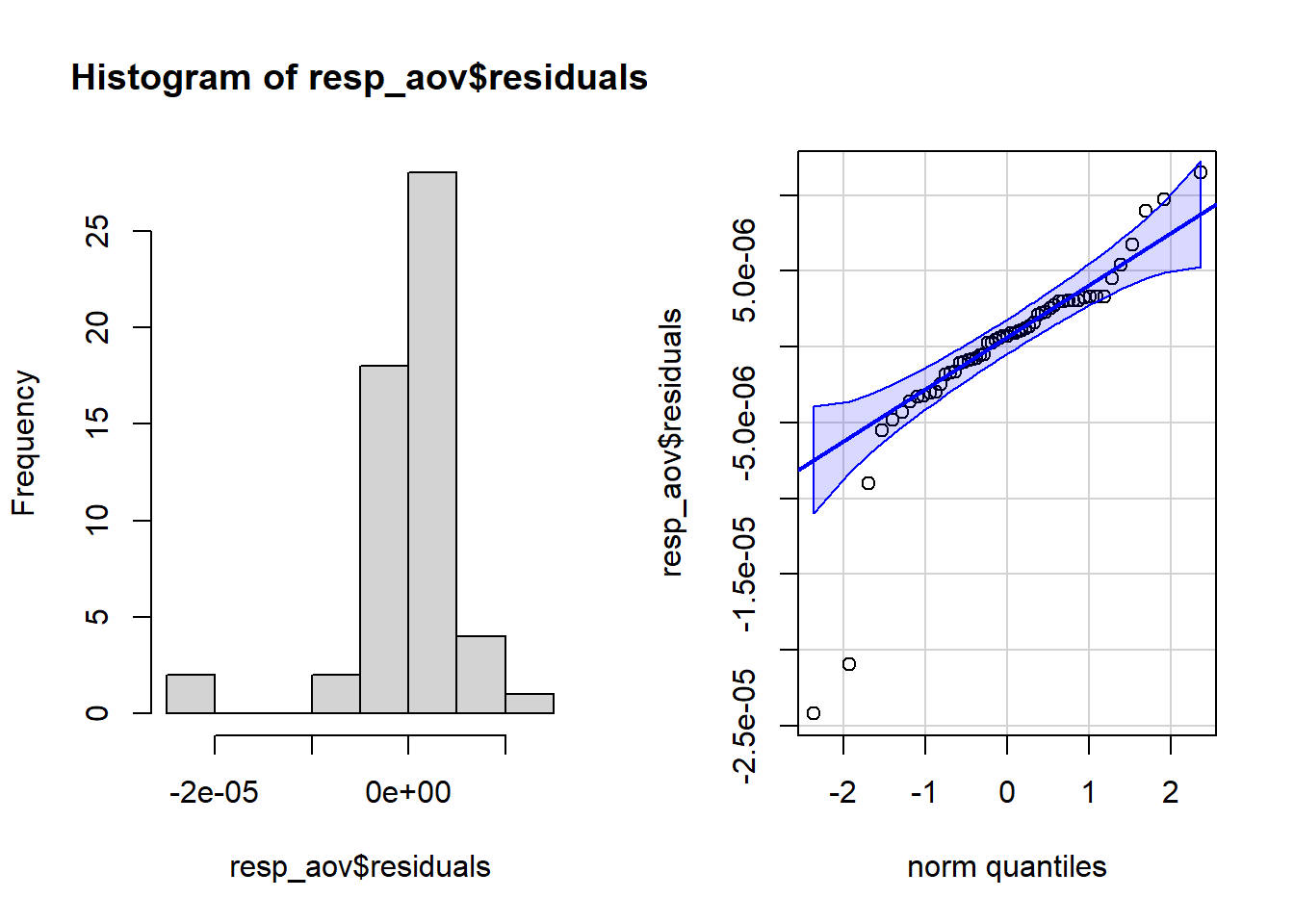
6.1.2 Data normality
resp_aov <- aov(massnorm_resp_rate ~ treatment, data = rates)par(mfrow = c(1, 2)) # combine plots
# histogram
hist(resp_aov$residuals)
# QQ-plot
qqPlot(resp_aov$residuals,
id = FALSE # id = FALSE to remove point identification
)
6.1.3 Boxplot
ggplot(rates) +
  aes(x = treatment, y = massnorm_resp_rate) +
  geom_boxplot() +
  theme(axis.text.x = element_text(angle = 45, hjust = 1))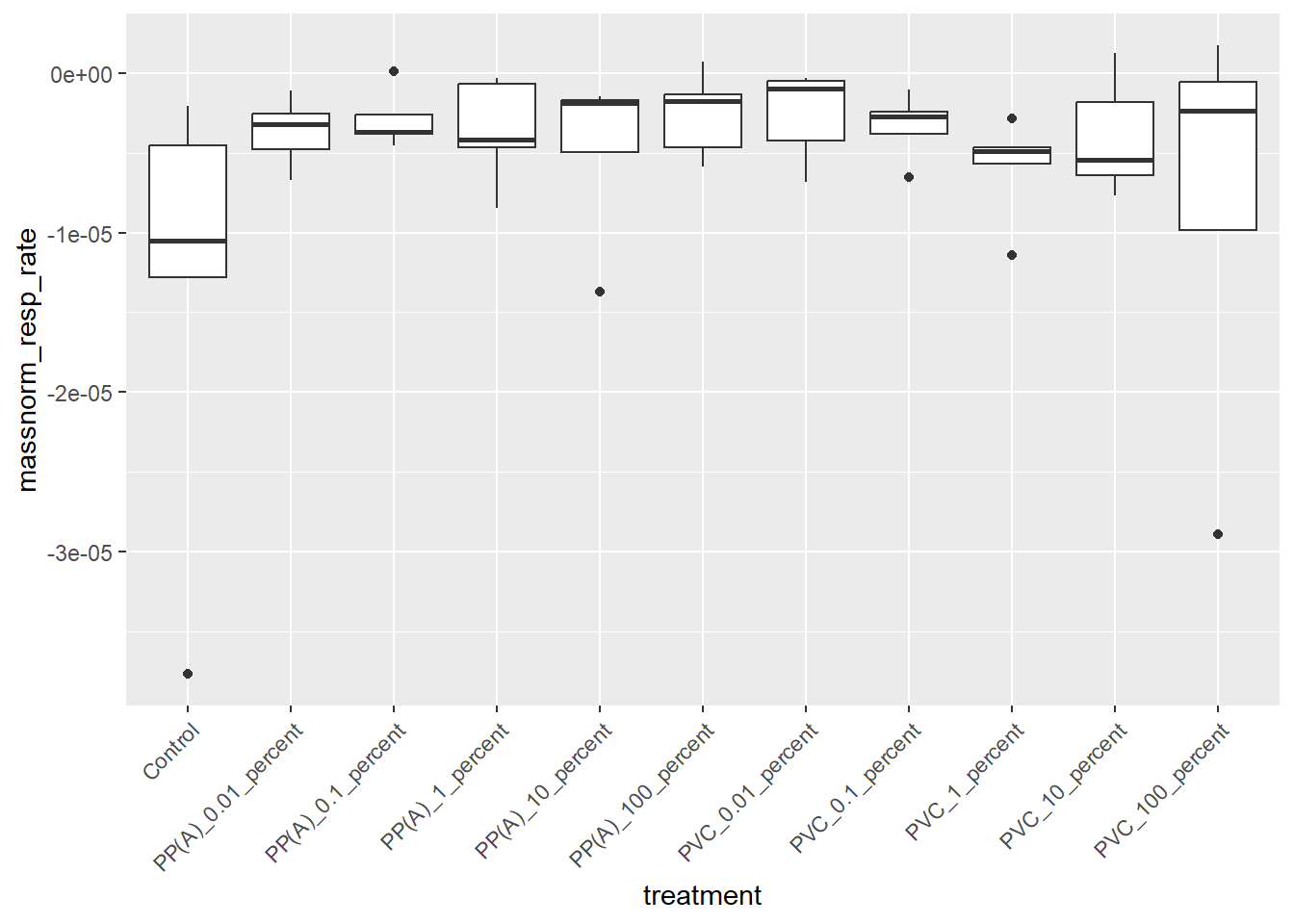
6.1.4 ANOVA
resp_aov <- aov(massnorm_resp_rate ~ treatment,
  data = rates
)

summary(resp_aov)
Df Sum Sq Mean Sq F value Pr(>F)
treatment 10 5.268e-10 5.268e-11 1.302 0.259
Residuals 44 1.780e-09 4.045e-11 6.2 Photosynthesis
6.2.1 First glimpse of data
ggplot(rates) +
  aes(x = treatment, y = massnorm_phot_rate, color = treatment) +
  geom_jitter() +
  theme(legend.position = "none")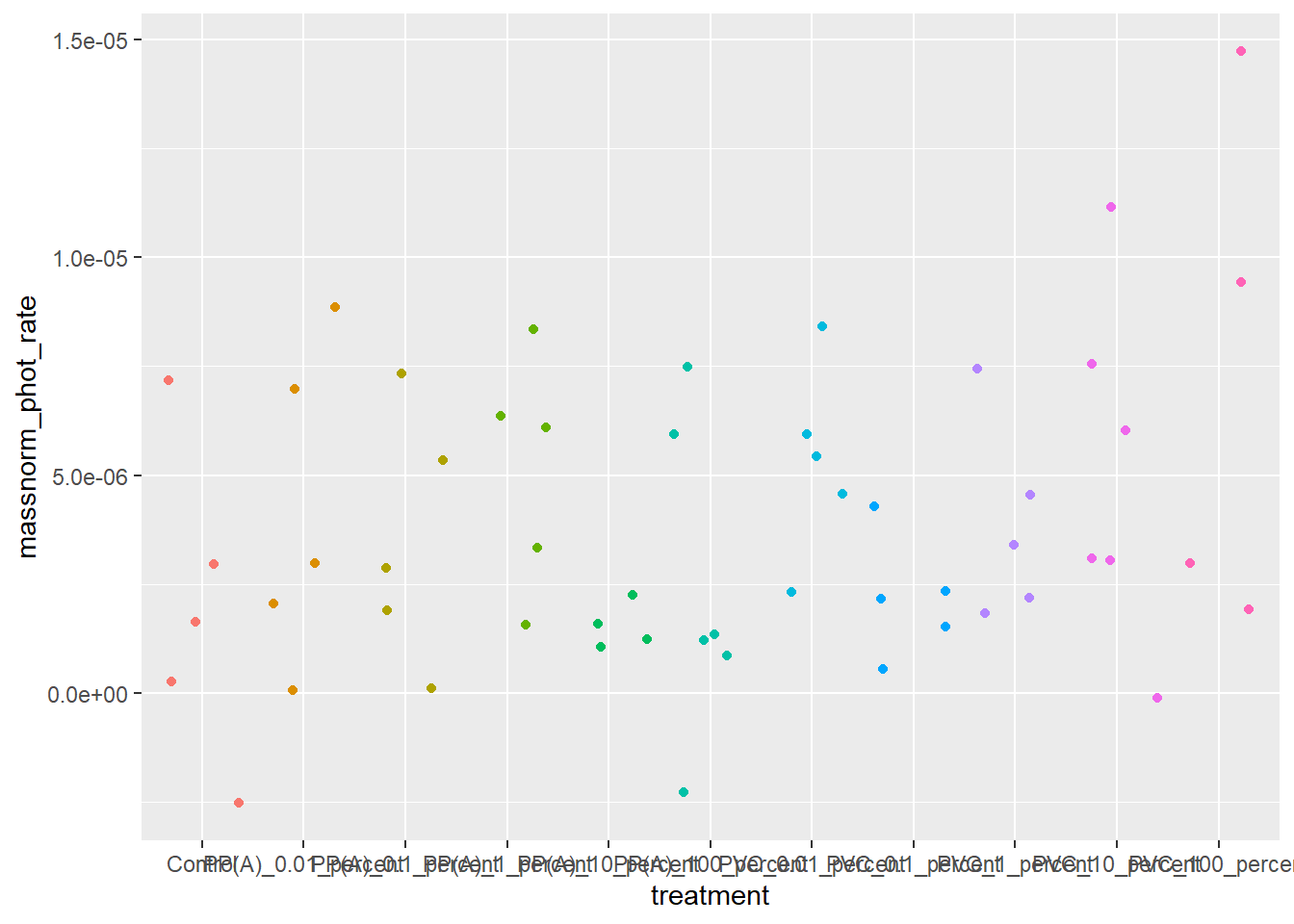
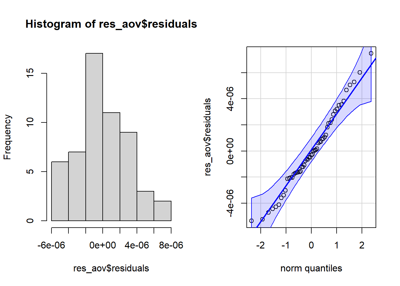
6.2.2 Data normality
res_aov <- aov(massnorm_phot_rate ~ treatment, data = rates)par(mfrow = c(1, 2)) # combine plots
# histogram
hist(res_aov$residuals)
# QQ-plot
qqPlot(res_aov$residuals,
id = FALSE # id = FALSE to remove point identification
)
6.2.3 Boxplot
ggplot(rates) +
  aes(x = treatment, y = massnorm_phot_rate) +
  geom_boxplot() +
  theme(axis.text.x = element_text(angle = 45, hjust = 1))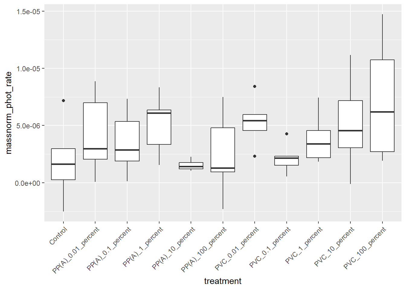
6.2.4 ANOVA
phot_aov <- aov(massnorm_phot_rate ~ treatment,
  data = rates
)

summary(phot_aov)
Df Sum Sq Mean Sq F value Pr(>F)
treatment 10 1.433e-10 1.433e-11 1.355 0.233
Residuals 44 4.652e-10 1.057e-11 7 Coming up next
Start the PAM Rapid Light Curve analysis
Extract RNA for gene expression of host anemone and symbiont dinoflagellate
8 Gaps & improvements
Important
We still need to be able to take the background signature of our filtered seawater using C18 SPME fiber extractions, preserve the fibers, and send them to the Saliu Lab for analysis
Note
We are limited to short exposures because of the 48 hour window we have to work with fresh leachate. We can get around this by making leachate in batches and doing water changes every 48 hours, but we will need larger stocks of microplastic with which to make the leachate if we want to pursue this